Dust coagulation
Dust coagulation in mcdust is done with a Monte Carlo approach rather than solving the Smoluchowski equation. We briefly explain the method here.
For details we refer the reader to Drążkowska et al 2013 and Zsom and Dullemond 2008 .
We follow representative particles and follow their evolution rather than tracking every single particle and its evolution. These \(n\) representative particles statistically represent \(N\) physical particles (\(n << N\)).
The representative particle \(i\) shares identical properties with \(N_i\) physical particles.
The total mass of physical particles in one swarm (\(M_{\mathrm{swarm}}\)) is given by
where \(m_i\) is the mass of the representative particle \(i\). The fundamental assumption here is that \(M_{\mathrm{swarm}}\) is the same for every swarm and is a constant over time. This means that if a particle grows (\(m_i\) increases), the number of particles it represents reduces (\(N_i\) reduces). This is a statistical effect and not a physical effect.
Collisions
In this framework, we assume that the representative particles themselves do not collide with each other (the collisions between the representative particles are too rare). The representative particles collide with physical (non-representative) particles whose history we do not track. We track only the representative particle and its evolution.
To perform a collision we choose a representative particle \(i\) and a physical particle represented by representative particle \(k\). The probability of a collision between particle \(i\) and particle \(k\) is given by
where V is the cell volume and \(K_{ik}\) is the coagulation kernel which is given by
with \(\sigma_{ik}\) being the geometric cross-section for the collision and \(\Delta v_{ik}\) being the relative velocity between particle \(i\) and \(k\).
The total collision rate for any pair can be computed by
Then, we can choose the represenative particle. The probability that the chosen particle is \(i\) is
The probability that this particle collides with a non-representative particle \(k\) is given by
Both these particles are chosen by drawing a random number.
The timestep between the collisions is determined as
where rand is a random number drawn from a uniform distribution between 0 and 1.
The subroutines that compute the collision rates and probabilities can be found in collisions.F90
The collisional outcomes between particles (sticking, fragmentation, erosion) is determined by their relative velocities. We explain the relative velocity formulation and the collisional outcomes below.
Relative velocities
The sources for the velocities of the particles taken into account are: Brownian motion, turbulence, radial and azimuthal drift and differential settling.
This is similar to the model described by Birnstiel et al 2010 . For the turbulent relative velocities, we use the prescription from Ormel and Cuzzi 2007 .
The implementation of the relative velocities in mcdust can be found in the relvels subroutine in collisions.F90
Collisional Outcomes
In the standard model the collisional outcomes are sticking, fragmentation and erosion. The outcomes are decided based on the relative velocities of the particles.
If the relative velocities are below a threshold velocity then we perform sticking. This threshold is the fragmentation velocity \(v_{\mathrm{frag}}\), which is an input parameter for mcdust.
If the relative velocities are above the fragmentation velocity then there are two outcomes, erosion and fragmentation, depending on the mass ratio of the particles.
The implementation of collisions can be found in the subroutine collision and subroutines therein, in the file collisions.F90
Sticking
In the case of sticking, we assume the physical particle \(k\) has been completely merged into the representative particle \(i\). As a result the mass of the particle \(i\) becomes
Since the mass of the represenative particle \(i\) increases, to conserve \(M_{\mathrm{swarm}}\), \(N_i\) reduces. This is a statistical effect and it can be balanced out with more collisions in the system. We refer the user to Zsom and Dullemond 2008 for a detailed discussion.
Fragmentation & Erosion
When the collision exceeds the fragmentation velocity the representative particle fragments. But there are two ways depending on the mass ratio between the particles. If two similar sized particles collide,
then this leads to a catastrophic fragmentation of both the particles which we term as fragmentation. But when a small particle collides with a larger particle, a catastrophic fragmentation is unlikely and
the likely event is that the small particle fragments and chips off a piece of the large particle. We term such an event as erosion. The threshold for the mass ratio between the particles can be set with the erosion_mass_ratio parameter in the setup.par file.
The default value is set to 10. We assume that the eroded mass is equal to the mass of the small particle.
For both the cases, there is a distribution of fragments as a result and this distribution is given by,
where \(\gamma = - \frac{11}{6}\) is a parameter derived from collisional models such as Dohanyi 1969 .
In the case of catastrophic fragmentation, the largest mass of the fragment is the mass of the largest collider and in the case of erosion, the largest fragment has the mass of the smallest collider.
Collision Optimization
Zsom and Dullemond 2008 introduced a fine-tuning parameter, denoted as \(dm_{\rm{max}}\), into the algorithm to group collisions and thereby accelerate computation. It limits the maximum mass ratio for grouping collisions by altering the collision rate of the particles.
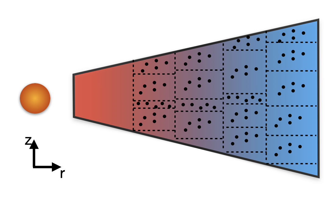
Adaptive Grid
Collisions happen between particles that are in close proximity to each other and, in order to resolve the physics properly in both high density and low density regions, we use an adaptive grid method to bin the particles.
The method works in such a way that each cell has the same number of particles which can be set by the parameter number_of_particles_per_cell in the setup.par file.
We show a schematic reprentation of the adaptive grid method below: