Data analysis and visualisation
In this notebook we show a way to make use of the helper python scripts and the routines to analyse and visualise data from mcdust.
We import routines from the script mcdust.py which is in the /scripts/ directory
The required pre-requisites for running the scripts are numpy, scipy, matplotlib, h5py, os, astropy, glob, tqdm, pandas
[1]:
from mcdust import Simulation, Plots
Reading data
The routines to read and store data from mcdust are stored in the Simulation() class, so let’s start by defining a variable
[2]:
sim = Simulation()
Next, to make use of the read function we need to establish the location of the data and give the same as an input.
[3]:
path='/your/path/to/data/directory'
sim.read(path)
 Reading paramters file from data files in /scratch/vaikundaraman/mcdust/outputs/data/
mcdust   v1.0
Authors : Dr Joanna Drazkowska, Vignesh Vaikundaraman, Nerea Gurrutuxaga
Please cite Drążkowska, Windmark & Dullemond (2013) A&A 556, A37
Reading data ...
100%|███████████████████████████████████████████| 42/42 [00:04<00:00, 9.42it/s]
Done!
/scratch/vaikundaraman/mcdust/scripts/mcdisk.py:208: RuntimeWarning: divide by zero encountered in true_divide
  self.taugrowth = 1/self.dtg/self.omegaK[:]
/scratch/vaikundaraman/mcdust/scripts/mcdisk.py:209: RuntimeWarning: divide by zero encountered in true_divide
  self.tmix = 1./(1e-3 * self.omegaK[:])
/scratch/vaikundaraman/mcdust/scripts/mcdisk.py:210: RuntimeWarning: invalid value encountered in true_divide
  self.rhog_mid  = self.sigmag/np.sqrt(2*np.pi)/self.Hg
We have read data into the object sim. The object sim contains the data of the swarms of the simulation in sim.swarms and the parameters of the simulation in sim.pars.
The object sim.pars contains the paramters of the simulation that was fed into setup.par to run the simulation. And along with those parameters, it also contains the number of swarms in the simulation nswarms and the number of outputs/snapshots of the simulation ntime.
The attributes of sim.pars can be seen below
[4]:
sim.pars.__dict__
[4]:
{'alpha_t': 0.001,
 'tgas': 280.0,
 'sigmagas': 800.0,
 'minr': 1.0,
 'maxr': 100.0,
 'a0': 1e-04,
 'vfrag': 1000.0,
 'rho_s': 1.2,
 'dtg': 0.01,
 'erosion_m_ratio': 10.0,
 't_end': 315581500000.0,
 'nr': 32,
 'nz': 16,
 'n_cell': 256,
 'nswarms': 131072,
 'ntime': 42,
 'eta': 0.05,
 'datadir': '/scratch/vaikundaraman/mcdust/outputs/data//',
 'alpha': 0.001}
The objectsim.swarms contains the id number of the swarms, radial location[AU], vertical height[AU], Stokes Number, grain size[cm], internal density [g/cm^3], radial velocity [cm/s], vertical velocity [cm/s].
The properties are stored in 2 dimensional arrays with indices [ntime,nswarms]. Along with these properties it also contains the mass of a whole swarm mswarm(g) and the times (yr) of the snapshots of the simulation.
[5]:
dir(sim.swarms)
[5]:
['St',
 '__class__',
 '__delattr__',
 '__dict__',
 '__dir__',
 '__doc__',
 '__eq__',
 '__format__',
 '__ge__',
 '__getattribute__',
 '__gt__',
 '__hash__',
 '__init__',
 '__init_subclass__',
 '__le__',
 '__lt__',
 '__module__',
 '__ne__',
 '__new__',
 '__reduce__',
 '__reduce_ex__',
 '__repr__',
 '__setattr__',
 '__sizeof__',
 '__str__',
 '__subclasshook__',
 '__weakref__',
 'calculate_properties',
 'describe',
 'grain_size',
 'idnr',
 'indens',
 'mass',
 'mswarm',
 'rcents',
 'rdis',
 'read_hdf5',
 'rwalls',
 'sigmad',
 'snapt',
 'velr',
 'velz',
 'zdis']
An overall basic statistics for the given simulation can be seen at a glance with sim.swarms.describe()
[6]:
sim.swarms.describe()
           mass [g]     Stokes Nr  grain_size [cm]
count  1.310720e+05  1.310720e+05    131072.000000
mean   8.931285e+01  4.464831e-03         0.448102
std    5.139990e+02  1.256053e-02         1.510780
min    5.026548e-12  2.409769e-07         0.000100
25%    4.523893e-11  4.614724e-05         0.000208
50%    6.936637e-10  9.578160e-05         0.000517
75%    5.245570e-06  1.044858e-03         0.010143
max    1.056346e+04  1.235100e-01        12.808906
There is also a routine sim.swarms.calculate_properties() to calculate the dust surface density sigma_d for the simulation.
Data Visualisation
The class Plots contains some routines to visualise the data. Currently there are 4 routines, Plots.scatter_all(), Plots.rz_scatter(), Plots.sigmad() and Plots.mass_dens_radial()
Scatter Plots
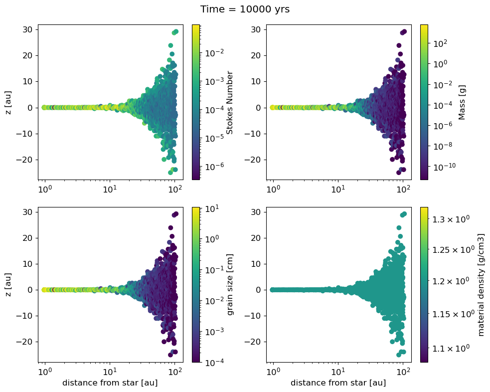
Scatter plots are helpful to visualise the different properties of the swarms.The Plots.scatter_all() visualises the default properties that are tracked in mcdust, namely, the Stokes Number, mass, grain size and internal density.
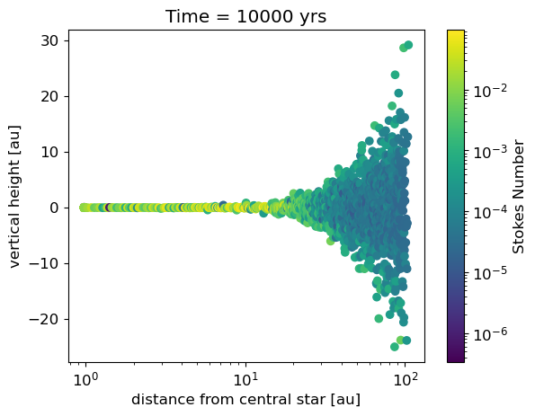
If you want to specifically look at one property, the Plots.rz_scatter() is helpful.
[7]:
Plots.scatter_all(sim.swarms, step=100)
#the argument step denotes the increment to print every nth variable. The default is 1.
[8]:
Plots.rz_scatter(sim.swarms,time=-1,step=100,scatter=sim.swarms.St,cbarlabel='Stokes Number')
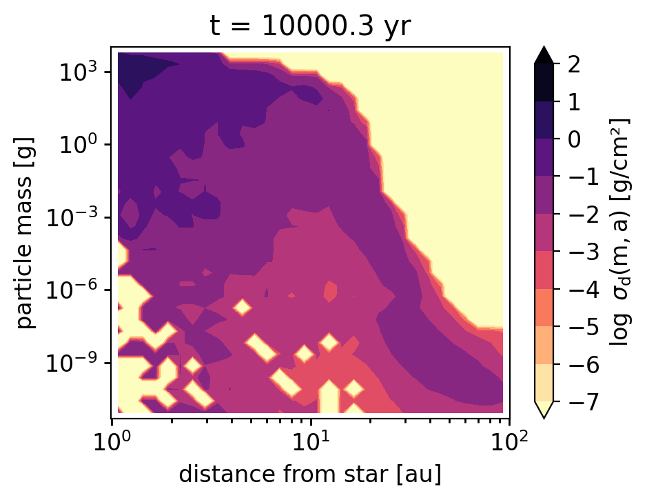
Dust surface density \(\sigma_d(\mathrm{m,a})\)
One can also quickly visualise the dust surface density with Plots.mass_dens_radial()
[9]:
Plots.mass_dens_radial(sim.swarms,sim.pars)
[ ]: